In the HMC Bee Lab (aka Ant Lab), we’re interested in the behavior of the tree-dwelling turtle ants, and have designed arenas to learn more about these creatures. Because we have hours and hours of data, we need a way to automate the extraction of useful information from our video data, for which our lab has built a pipeline to determine certain regions of interest (ROIs) where we track the flow of ants. In previous experiments, the arena consisted of simple rectangular and pentagonal regions, which were all marked with a red sharpie.
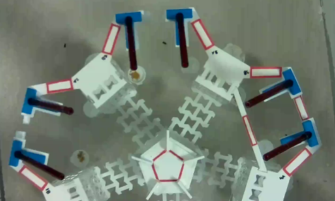
Figure 1: Arena for 2019 turtle ant experiments
In this year’s experiments, however, we wanted to study the turning biases of turtle ants in a more natural tree-like setting, so the lab designed a new tree structure consisting of more complex Y junctions. A large part of my project was to detect these new ROIs, and consistently label them across all of our videos.
Figure 2: Arena for 2021 turtle ant experiments
I tackled the task of finding the locations of the ROIs in OpenCV using the following process. First, I took a frame from the video, applying a threshold to separate out the lighter tree structure from the darker background. Once I singled out the tree, I skeletonized it, reducing it to a 1 pixel wide representation. With the skeletonized image, I was able to find the branching points (the centers of each ROI) using the sknw library, which transformed the tree into a network. Now, the tricky part: I needed a way to find the vertices of the ROIs based on the centerpoints I found. I did this by drawing a large circle around the centerpoints, then overlaying these circles with the contour of the tree and finding the points of intersection. Finally, I used opencv’s convex hull function to properly connect the vertices.


Figure 3a: Zoomed in image. Figure 3b: Skeletonized image of 3a with branching point marked in yellow. Figure 3c: Circle overlaid with contour of 3a, with vertices of ROI marked in green.

Figure 4a: Detected vertices drawn in green.

Figure 4b: Drawn and labelled ROIs
Although we’ve found and connected the vertices for the ROIs, we still needed to consistently label them across videos to recognize which ROI is being referred to. I accomplished this with the help of ARTags, a fiducial marker system. These tags, which we taped onto several food platforms of trees, serve as mini QR codes which the computer can easily recognize. Using these tags as points of reference, I warped the query image we want to label to match the perspective of a pre-labelled reference image using homography. With the two images aligned, I then matched the center points of the ROIs in the query image to the center points of the ROIs in the reference image, using distance as a heuristic. This way, the labelling would be consistent across all videos. Finally, I mapped the ordering of the ROI centers to match the labelling scheme the lab uses.
In addition, I needed to label the edges consistently in order to know which direction an ant travels as it enters and exits the ROI. I did this by finding the longest edge of the ROI, which always corresponded to the side segment, and shifted the vertices so that the long edge always came first using numpy’s roll function. However, the labels for the important edges (edges where ants actually walk across), were still inconsistent as there are two types of junctions, depending whether the smaller branch goes to the left or right. Since we know which ROIs are left and which are right from the labelling, I simply shifted the right junction vertices again so the significant edges lined up for all junctions. As shown in Figure 5, edge 1 corresponds to the base of the tree, edge 3 corresponds to a left turn, and edge 5 corresponds to a right turn.

Figure 5: Final detected and labelled ROIs
Now, we’re able to accurately detect ROIs over every single junction, even if the tree is slightly bent or warped. In addition, each ROI and its edges are consistently labelled, allowing us to consolidate and compare data across all the different videos, without having to do the tedious task of manually labelling each junction. With this pipeline, we will be able to extract data about ant turning choices at a much larger scale and in a more natural context with the colony level experiments.
Further Reading:
OpenCV’s aruco tag tutorial: https://docs.opencv.org/4.5.2/d5/dae/tutorial_aruco_detection.html
OpenCV’s contour tutorial:
https://docs.opencv.org/3.4/d4/d73/tutorial_py_contours_begin.html
OpenCV’s list of perspective transform functions:
https://docs.opencv.org/3.4/da/d54/group__imgproc__transform.html
Media Credits:
Figure 1: Picture taken from our lab’s 2019 experiments
Figure 2: Picture taken from our lab’s 2021 experiments (courtesy of Simon and Carter)
Figure 3,4,5: Computer generated images from lab’s videos
No comments:
Post a Comment