Skeletonization of Trees

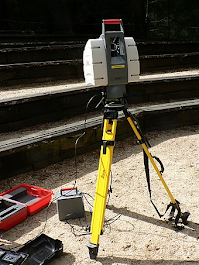
Example of a LiDAR laser scanner.[1]

When you take a picture of a tree, you generally get a beautiful - but fairly unhelpful - image of a trunk and a lot of leaves. If it’s maybe winter and the leaf cover has fallen, it’s still often hard to discern the exact branching structure - branches further away from the camera appear smaller, or are obscured by other branches, etc. Which brings us to the question - how can we accurately capture geometrical and spatial information about a tree? A fairly new but promising technique is laser scanning - using lasers to find the distance to your object of interest, and using those distances to create a cloud of points representing a 3D model of that object, otherwise known as a point cloud. The laser is often used in conjunction with digital photography in order to create a 3D image of the object. That 3D image, composed of millions of individual pixels, can reveal volumes of information about a tree - if we know how to use it correctly. 

When thinking about how to store information about a tree, there are several possible ways to go about it - and there’s never really a wrong or right answer, it just depends on what you’re hoping to achieve. One such structure is a “skeleton” - essentially a collection of many connected lines that represent the branching structure of a tree and the dimensions of its branches. Its simplicity offers several advantages - during the construction of a skeleton (otherwise known as the skeletonization of the tree), any noisy or imperfect points are eliminated, and only the branching structure, branch lengths and branch diameters are extracted from a large dataset.

Which brings us to the question - how can we construct this skeleton? There exists an algorithm called SkelTree (short for Skeletonization of Trees) that extracts the skeleton from a point cloud by using one main attribute called the local elongation direction. Simply stated, a branch’s elongation direction is the direction in which it grows, or elongates. If you simplify a tree branch/limb into a cylinder, the elongation direction is simply the direction that the height of the cylinder extends in. In order to create the skeleton, the points are shrunk down in the direction perpendicular to the elongation direction until they form a line running through the middle of the original tree limb.

Diagram of a branching junction of a point cloud. Red regions signify non-branching regions and yellow regions signify branching regions. [2]

This results in lines centered locally within each limb of the point cloud tree. The elongation direction is integral to the algorithm because it reveals several aspects of the tree on a local and global scale - for example, it gives us branching points, branch lengths, and branching angles. Any point at which the elongation direction changes can be interpreted as a branching point, and the angle at which it changes gives us the branching angle. Since the calculation required to obtain the elongation direction is fairly straightforward, and it reveals a lot of information about the tree, computing the skeleton using the elongation direction alone results in a highly efficient algorithm.

(a) simple 2D tree. (b) simple 2D tree with its skeleton. (c) isolated skeleton of 2D tree. (d) branching points of the tree.[3]

Segment of point cloud divided into five octree-cells.[4]

So how does the algorithm find this integral piece of information at each limb of the tree? Our first step is to compute an octree-graph. Essentially, the point cloud of the tree is chopped up into numerous small cubical cells that share at least 1 side, called octree-cells. The center of each octree-cell is determined to be a vertex in the octree-graph. Neighboring vertices are then connected by an edge if the point cloud passes through the vertices’ corresponding cells’ shared side, meeting the robustness criteria specified by the algorithm. The robustness criteria essentially evaluate whether enough points in the point cloud pass through the current cell side of interest. The edge is then labelled by a set of 3 numbers representing its cartesian direction (for example, (-1, 0, 0), which represents the “left” side of the cell). This results in an octree-graph: a set of interconnected edges and vertices derived through octree-cells. The way the edges are computed are actually the way to compute the local elongation direction - hence, each edge represents the local elongation in that area. The graph now represents the surface of the object and contains the local elongation direction at any given point in the tree.

The next step of the algorithm is to compute the skeleton from the octree-graph. This is done by merging specific pairs of vertices (the corners at which edges meet). Pairs of vertices are chosen to be merged based on whether or not they preserve the elongation direction of the tree. Vertex pairs are merged repeatedly until a skeleton appears from the octree-graph.

Octree-graph reduction rules.[5]

The figure above illustrates the way that the octree-graph is reduced to a skeleton. The lower part of the figure represents the different octree-cell cases that are then reduced to the basic rule, which is illustrated in the top half of the figure, ultimately leading to a skeleton.

The final step of the algorithm is to embed the skeleton in the original point cloud using the pre-existing correspondence between the vertices of the skeleton and specific sets of points. The result is a skeleton composed of vertices and edges that are centered locally within the point cloud, allowing the user to access a certain location in the point cloud and obtain information from the skeleton at that location. This easily accessible data means that tree skeletonization has a variety of applications - from analyzing a particular tree species’ branching patterns, to understanding arboreal ant movements (one of the Bee Lab’s current projects), the possibilities are boundless.

Further Reading:
1. Bucksch, Alexander Klaus. “Revealing the Skeleton from Imperfect Point Clouds.” TU Delft Repositories, 2011, repository.tudelft.nl/islandora/object/uuid%3A45a7a7ac-a658-4274-9899-6f7e34d63334.

2. Calders, Kim, et al. “Terrestrial Laser Scanning in Forest Ecology: Expanding the Horizon.” Remote Sensing of Environment, vol. 251, 15 Dec. 2020, p. 112102., doi:10.1016/j.rse.2020.112102.


Media credits:
[1]: Public domain image. https://en.wikipedia.org/wiki/Lidar

[2]: Figure 2.4 from Alexander Klaus Bucksch. 2011. ”Revealing the skeleton from imperfect point clouds”. https://repository.tudelft.nl/islandora/object/uuid%3A45a7a7ac-a658-4274-9899-6f7e34d63334

[3]: Figure 2.3 from Alexander Klaus Bucksch. 2011. ”Revealing the skeleton from imperfect point clouds”. https://repository.tudelft.nl/islandora/object/uuid%3A45a7a7ac-a658-4274-9899-6f7e34d63334

[4]: Figure 4.1 from Alexander Klaus Bucksch. 2011. ”Revealing the skeleton from imperfect point clouds”. https://repository.tudelft.nl/islandora/object/uuid%3A45a7a7ac-a658-4274-9899-6f7e34d63334

[5]: Figure 3.11 from Alexander Klaus Bucksch. 2011. ”Revealing the skeleton from imperfect point clouds”. https://repository.tudelft.nl/islandora/object/uuid%3A45a7a7ac-a658-4274-9899-6f7e34d63334