When you look at the name random forest for the first time, you might not think that there is a relationship between this term and machine learning at all. However, random forest proves to be a really powerful machine learning classification model. A good classification model would take in a sample and predict which of several categories it fits best. A good example of classification learning would be the Bee Lab’s flower mapping project, which the project I am currently working on. The project tries to find flowers within drone images, and then identify the flowers by species. Out of many classification models initially tested by members of the Bee Lab, we ended up using the random forest because of its high performance. This blog post will briefly explain two reasons why random forest is so powerful, and yes, you guessed them: the two reasons are “random” and “forest”. In this blog post, you will learn what random forest is and how “random” and “forest” together make random forest a powerful classification model.
1. Decision Tree Model
Before embarking on a lengthy discussion of the random forest model, let’s talk about the simpler decision tree model, as random forest is made up of many decision trees. In other words, many decision trees form the “forest” part of the random forest model. By itself, a decision tree is also a classification model that works well in many scenarios.
The way it works is shown in the image below. Here we are training a model on predicting whether a person will accept a certain job offer based on three features: (1) whether the salary is at least $50,000; (2) whether the commute takes more than an hour; (3) whether the workplace offers free coffee. Based on the training data, the decision tree will choose one of the three features that has the highest distinguishing ability to be put at the root of the tree. By highest distinguishing ability, I mean the ability of a feature to categorize samples into either “accepts” or “decline” the most correctly. In this case, feature (1) has the highest distinguishing ability, so it’s put at the root of the decision tree. Then it goes on to further distinguish those samples who answer yes to the first feature, by selecting the root of the corresponding subtree in the same way as choosing the root of the whole tree - based on distinguishing ability. Note that by “answer[ing] yes to the first feature”, I mean that, in our case, a job offer has a salary of at least $50,000. The tree goes on until it exhausts all the features given in the dataset, which is when we say the training process for a decision tree is complete.
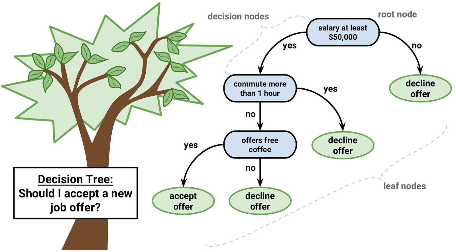
[1] A decision tree example.
The reason we want to use the distinguishing ability to choose roots is obvious: this way, we can most speedily narrow down to find samples who require answers to later questions. In other words, since the salary feature has the highest distinguishing ability, if we put it at the top, we can eliminate the most number of nodes correctly and efficiently, without the need to worry about the samples that say “no” to the salary question. In contrast, if we were to use the coffee feature at the top, then we would probably still need to include the salary question on both “yes” and “no” sides of the tree because the coffee question is not overarching enough. Using distinguishing ability to choose the roots of subtrees means that subtrees always only need to process the minimal number of samples during training. Similarly, each sample only needs to go through minimal number of nodes for classification, speeding up its prediction process as well.
This is of course a pretty good trait, making decision tree’s training and classification time-efficient. However, it can also be a huge problem. Here is the contradiction: the training is missing on those samples whose answers to features do not fit the usual pattern. More concretely, in our example, there might be some individuals who would say yes to a job that has a salary of less than $50,000 USD. Even though decision tree models are very fast to train and predict, they will fail pretty easily in these cases. Therefore, we need a better model based on decision trees!
2. Bagging ensemble: Power of the majority
Now that we have discussed the decision tree by itself, we will briefly go through another reason why random forest is powerful: bagging ensemble. As you might guess from the title of this section, bagging ensemble is what renders random forest with the “random” magic power.
Bagging, as one of the two most popular ways to ensemble, means to train a bunch of individual models in a parallel way. [2] Note that each model is trained on a random subset of the data, and each model’s training set does not overlap with other individual models’ training set. This makes each model a weak classifier -- less training data and features generally means lower accuracy -- but the final decision is made by the majority vote of all these models. Bagging ensembles use the majority vote of many decision trees to get a better prediction performance. Simply put, this is the ancient Greek Democracy practiced in machine learning: the majority rules!
 .
.The power of this method stems from the belief that the majority decision of a bunch of weak classifiers transcends the decision of one single strong classifier. This makes sense. These decision trees are individually weak and can make the mistake of missing training on samples that do not follow the usual patterns, as mentioned in section (1). However, when combined, they can correct each other’s mistakes and actually cover more of the training data, as long as we have a large enough training dataset and a large enough feature set.
3. Random Forest: the power of “Random” and “Forest”
Last but not least, let’s see how we combine the power of ensemble and decision trees to make the powerful random forest. Indeed, random forest is a bunch of decision trees, but there is a really important nuance. In addition to only getting a subset of training data for each decision tree, each tree only gets a subset of all features available.
Why is that important? Doesn’t that further weaken the strength of each individual classifier? Yes, but this is actually what we have to do: to make majority votes work, we have to make sure that voters are unbiased and do not collude with each other. In more mathematical terms, we need to randomize the roots of each decision tree and its subtrees. Using only a subset of training data and features makes sure that each weak classifier can only decide the order of distinguishing abilities according to the limited training data and features available to it. This enables us to ensure that the individual decision tree models are uncorrelated, and thus more unbiased. This is another “randomness” in addition to the “randomness” from selecting random training sets for the decision trees. If you would like to read more about this, the picture below from this article visually explains how bagging works in the random forest model.

[3] The magic🔮 of the randomness.
Then you might wonder how big a subset of all features each decision tree should get: this is a fantastic question! Indeed, this is actually specified by the depth of decision trees, a hyperparameter of the random forest model. So the short answer is: I don’t know, but random forest can learn to find the hyperparameter too! For example, you can use grid search to search for optimal parameters given a parameter grid.
In a nutshell, the random forest model works well because of the magic of “random” and “forest”! To remind you again, the power of “randomness” comes from selecting random subsets of training data and features for each decision tree, and the power of “forest” comes from having a bunch of decision trees!
Further reading:
Breiman, Leo. “Random Forests”. Machine Learning, 45, 5–32, 2001. Kluwer Academic Publishers. https://link.springer.com/content/pdf/10.1023%2FA%3A1010933404324.pdf
An example of random forest used in biomedical contexts: Kulkarni, S., Chi, L., Goss, C., Lian, Q., Nadler, M., Stoll, J., Doyle, M., Turmelle, Y., & Khan, A. (Accepted/In press). Random forest analysis identifies change in serum creatinine and listing status as the most predictive variables of an outcome for young children on liver transplant waitlist. Pediatric transplantation. https://doi.org/10.1111/petr.13932
Media credits:
[1] How Decision Tree Algorithm Works by Rahul Saxena, https://dataaspirant.com/how-decision-tree-algorithm-works/
[2] Basic ensemble learning by Lujing Chen, https://towardsdatascience.com/basic-ensemble-learning-random-forest-adaboost-gradient-boosting-step-by-step-explained-95d49d1e2725
[3] Cartoon drawing by Illustration Olga Kuevda, https://www.dreamstime.com/people-voting-ancient-greece-cartoon-male-citizens-placing-pebbles-urn-funny-vector-illustration-democracy-origins-image142323276
No comments:
Post a Comment